Profile a Community with BLAST
The above diagram shows the process of getting a community profile from a BLAST run against a DB of choice. The choice of DB is up to the user, but any DB that provides a NCBI taxon_id can be used. Such DBs include the ones provided by NCBI (e.g. nt, nr, viral) as well as Uniprot (SwissProt, TrEMBL).
The community profile will use an assembly and we want to assign each of its contigs to taxon. This can be done a BLAST output and a series of scripts that ends with the lca command of the taxon_utils script (taxon-utils - Taxonomy Utilities). lca stands for last common ancestor, which indicates that given a number of taxa, we try to resolve the taxon they all have in common. This can be of any level, from a specific strain to a kingdom, such as Bacteria.
There a cases when there’s no lca that can be resolved and this is due to the way NCBI taxonomy is structured, with multiple top levels, such as cellular organisms, viruses and so on.
Note
Other DB may provide the taxon_id from NCBI, but this should be checked by the user
Considerations
Since the assembly of a metagenome is a time consuming process, the assembly from the hmmer-tutorial tutorial will be used. We’ll try to use all results from the nt DB from NCBI, as well as separate viruses and cellular organisms and resolve the lca for those annotations separately.
Another thing to consider is how to filter the annotations. That’s up to the user to decide which suits the specific task, but these options will be examined:
- filter based on a static threshold, such as > 50 bitscore (using filter-gff values)
- filter based on a dynamically chosen value, keeping only the X top options (using filter-gff sequence)
- filter based on overlap (using filter-gff overlap)
The results may differ, and they are listed from the fastest to the slowest.
Requirements
MGKit should be installed and its scripts can be run from the command line. Refer to the installation for this, but it’s assumed that it was installed with:
$ pip install mgkit[full]
Moreover, the tutorial makes use of UNIX command line utilities, so a version of GNU/Linux, BSD or MacOS X should be used to run this tutorial. *BASH is expected to be the shell running.
The following should be installed as well:
- BLAST+ (blastn will be used)
- ncftp (used to download the NCBI nt DB)
MacOS X
The software requirements can be installed with homebrew, using the following command:
$ brew install ncftp blast
Download Data
Assembly
TODO
NCBI nt
We’ll be using the NCBI nt which will be stored in the ncbi-nt directory. If a copy is already somewhere, just create a symbolic link to that directory, for example:
$ ln -s path-to-the-db ncbi-nt
Otherwise, a copy can be downloaded and prepared with the following commands:
1 2 3 4 5 6 | $ mkdir ncbi-nt
cd ncbi-nt
ncftpget ftp://ftp.ncbi.nlm.nih.gov/blast/db/nt*.gz
for x in *.tar.gz; do tar xfvz $x ;done
rm *.tar.gz
cd ..
|
ID to Taxonomy
The following file contains the taxon_id for all the IDs in the NCBI nt DB. It will be used to add taxonomic information before running the lca step:
$ wget ftp://ftp.ncbi.nih.gov/pub/taxonomy/accession2taxid/nucl_gb.accession2taxid.gz
NCBI Taxonomy
This can be installed using the following script included in MGKit:
$ download-taxonomy.sh
Which will create a file called taxonomy.pickle
Community Profiling
To make the tutorial faster, we’ll filter the assembly file to include only contigs of at least 500bp:
1 2 3 4 5 6 7 | $ python - <<END
from mgkit.io import fasta
with open('final-contigs-filt.fa', 'w') as f:
for name, seq in fasta.load_fasta('final-contigs.fa'):
if len(seq) >= 500:
fasta.write_fasta_sequence(f, name, seq)
END
|
BLAST
The blastn command will be used to search for similar sequences in the NCBI nt DB. The following command will create a tab separated file with the results:
$ blastn -query final-contigs-filt.fa -db ncbi-nt/nt -outfmt 6 -out assembly-nt.tab -evalue 0.001
Convert into a GFF
The following command will create a GFF file from the BLAST output:
$ blast2gff blastdb -i 3 -r assembly-nt.tab assembly-nt.gff
We’re using the blastdb command of the blast2gff command, since it gives more control over the way the header file is formatted:
gi|118501159|gb|CP000482.1|
At the moment, the header format of the NCBI nt DB is a | (pipe) list that contains two type of identifiers. The first element is gi, to indicate that the following element (second) is the GI identifier that it’s being retired in September 2016. The third is indicates the DB from where the other ID originates from (GenBank in this case) and the fourth is the identifier that we’ll use.
By default blast2gff blastdb used the second element (118501159) of the header as gene_id, so we use:
- -i 3 to instead use the fourth element (CP000482.1) as gene_id
- -r will remove the versioning information from the gene_id, so CP000482.1 will become CP000482
The reason for this is that the file containing the taxon_id for each identifier is better used with a fourth element of the header without the versioning information.
Adding the Taxonomic Information
The add-gff-info addtaxa command allows to insert taxonomic information (in the GFF taxon_id attribute) into the GFF file. This step integrates the content of the nucl_gb.accession2taxid.gz file with the GFF file. The structure of this file is:
ACCESSION ACCESSION.VERSION TAXONID GI
Warning
this command has to load all the GFF in memory, so a high memory machine should be used (~30GB). The GFF can be split into smaller files to save memory and the subsection here will describe the process.
Since we used the ACCESSION as gene_id, we need to edit the file to pass it to the add-gff-info addtaxa command -t option. This can be don on the fly and the following command adds information to the GFF file created:
$ add-gff-info addtaxa -t <(gunzip -c nucl_gb.accession2taxid.gz | cut -f 1,3) -e assembly-nt.gff assembly-nt-taxa.gff; mv assembly-nt-taxa.gff assembly-nt.gff
The -t option is the file that can contains the taxon_id for each gene_id, the script accept a tab separated file. After the this we rename the output file to keep less files around. The -e option was used to remove from the output file any annotation for which a taxon_id was not found. Since we need them for the LCA later, it makes sense to remove them before filtering.
Reduce Memory Usage
First we need to split the assembly-nt.gff file, with a good option being using the split command in Unix. The following command will create the files:
$ split -l 1000000 -d assembly-nt.gff split-gff
This command will create 12 GFF files (of at most 1 milion lines each), whose names start with split-gff. Since we split the files we can use a loop to add the taxonomic information to all of them:
1 2 3 | $ for x in split-gff*; do
add-gff-info addtaxa -t <(gunzip -c nucl_gb.accession2taxid.gz | cut -f 1,3) -e $x $x-taxa;
done
|
This reduces the memory usage to ~2.5GB, but it takes longer to re-read the nucl_gb.accession2taxid.gz 12 times. There are way to parallelise it, but they are beyond the scope of this tutorial.
After the command has finished running, the content of the files can be concatenated into a single file again and delete the split files:
$ cat split-gff*-taxa > assembly-nt.gff; rm split-gff*
Filter the GFF
As mentioned we’ll provide three different way to filter a GFF, before passing it to the script that will output the lca information. This way we can compare the different filtering strategies.
Filter by Value
Let’s assume a scenario where we’re working on reads or very short contigs. We may decide to use a threshold, so the filtering is fast, but doesn’t compromise the quality of the assignment. This can achieved using the filter-gff values command:
$ filter-gff values -b 50 assembly-nt.gff assembly-nt_filt-value.gff
The command will read the GFF file and keep only the hits that are greater than or equal to 50, which we’re assuming is a good compromise for the assignment. This filtering strategy has the advantage of operating on a per-annotation basis, so the memory usage is low and no grouping or calculation is required.
Filter Dynamically
While the above can be give good results, we can think of cases where the number of hits that pass that threshold may be high (e.g. a conserved sequence in multiple organisms). In this case a more sensible choice would be to keep only the hits that are in the top 5-10% of the hits on that contig, all those over the median, mean or any other threshold based on the distribution of a sequence’s hits. The filter-gff sequence command can be used to filter the GFF:
$ filter-gff sequence -t -q .95 -c ge assembly-nt.gff assembly-nt_filt-sequence.gff
The options used will keep only the hits that have a bitscore (evalue and identity can also be used) greater than or equal to the top 5% of the bitscore distribution for that contig.
This threshold will include also contigs that have only one hit (that’s the reason to use -c ge instead of -c gt). We also assume that the input GFF is sorted (-t option) by contig name, to use less memory.
Filter Ovelaps
Let’s assume that in some cases the we think there may be cases where the contig contains regions that different rates of conservation. The first filter may keep too many taxa with similar sequences in a portion of the contig, while the second one may not provide enough coverage of the contig, keeping only the very best hits.
In this case, we can use the filter-gff overlap command to keep of all overlapping hits only the best one. And since we want to make sure that we still have good homology, we could still filter by value the hits, before that filter.
The following command will make that type of filtering:
$ filter-gff values -b 50 assembly-nt.gff | sort -s -k 1,1 -k 7,7 | filter-gff overlap -t -s 1 - assembly-nt_filt-overlap.gff
We just chained the filtering from the values command, keeping only annotations with at least 50 bitscore and passing it to the sort command. This passage is not necessary it the the -t option is not used with filter-gff overlap, but it uses less memory by pre-sorting the GFF by contig/strand first, since the filter-gff overlap works on each strand separately. We also used the -s options to trigger the filter for annotations that overlap for as much as 1 bp.
More information about this type of filter can be found in simple-tutorial and filter-gff - Filter GFF annotations.
Getting the Profile
We’ll have 3 GFF files ending in final.gff, one per each type of filtering, that contain the taxon_id for each annotation they contain.
Note
these files are available at this page if you want to skip
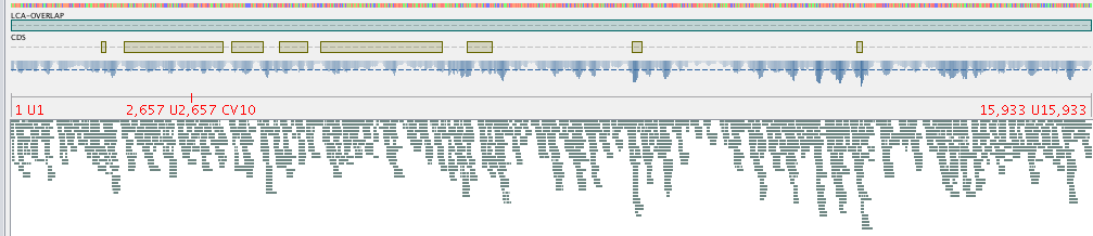
Since the filtered files are available now, we can create a file that contains the LCA assignments. We can ouput 2 type of files (see taxon-utils - Taxonomy Utilities), but for the purpose of this tutorial, we’ll get a GFF file that we can also use in a assembly viewer. The command to create them is:
1 2 3 | $ for x in *filt-*.gff; do
taxon_utils lca -v -t taxonomy.pickle -r final-contigs-filt.fa -s -n `basename $x .gff`-nolca.tab -ft LCA-`echo $x | egrep -o 'value|overlap|sequence' | tr [:lower:] [:upper:]` $x `basename $x .gff`-lca.gff;
done
|
The options used are:
- -t to direct the script to the taxonomy that we already downloaded
- -r to output a GFF with one annotation per contig that covers the whole sequence
- -s indicates that the input is sorted by reference sequence
- -n outputs a tab separated file with the contigs that could not be assigned
- -ft is used to change the feature type column in the GFF, from the dafault LCA to one which includes the type of filtering used
The file ending in -nolca.tab contain the contigs that could not be assigned, while the files ending in -lca.gff contain the taxonomic assignments, with the taxon_id pointing to the assigned taxon identifier, taxon_name for the taxon scientific name (or common name if none is found) and lineage contains the whole lineage of the taxon.
Using Krona
Besides having a file with the assignments and a GFF that can be used in Tablet, a quick profile can be produced using Krona and its associated Krona Tools. To produce a file that can be used with Krona Tools the -k can be used with the taxon_utils lca command. An additional option is to give the tool the total number of sequences in the assembly with the -kt option, to have a complete profile of the assembly:
1 2 3 | $ for x in *filt-{overlap,sequence,value}.gff; do
taxon_utils lca -v -t taxonomy.pickle -k -kt `grep -c '>' final-contigs-filt.fa` -s $x `basename $x .gff`-lca.krona;
done
|
To the -kt option was passed the total number of sequences (just used grep to count how many headers are in the fasta file).
The produced files with krona extension can be the be used with the ktImportText (or ImportText if Krona Tools were not installed). The -q option of the script must be used:
1 2 3 | $ for x in *.krona; do
ktImportText -q -o `basename $x .krona`.html $x;
done
|
This will create an HTML file for each one that can be read in a web browser.