Tutorial - Exploring the Data
The following section requires that:
- the tutorial has been completed
- the data from it is in the same directory
In alternative the data required to run this example can be download from figshare and uncrompressed.
Imports
[1]:
from __future__ import print_function

#Python Standard Library
import glob
import pickle
import sys
import functools
#External Dependencies (install via pip or anaconda)

# Check if running interactively or not
import matplotlib as mpl # http://matplotlib.org
# from:
# http://stackoverflow.com/questions/15411967/how-can-i-check-if-code-is-executed-in-the-ipython-notebook
# and
# http://stackoverflow.com/questions/15455029/python-matplotlib-agg-vs-interactive-plotting-and-tight-layout
import __main__ as main
if hasattr(main, '__file__'):
    # Non interactive, force the use of Agg backend instead
    # of the default one
    mpl.use('Agg')

import numpy # http://www.numpy.org
import pandas # http://pandas.pydata.org
import seaborn # http://stanford.edu/~mwaskom/software/seaborn/
import scipy # http://www.scipy.org
import matplotlib.pyplot as plt


#MGKit Import
from mgkit.io import gff, fasta
from mgkit.mappings import eggnog
import mgkit.counts, mgkit.taxon, mgkit.snps, mgkit.plots
import mgkit.snps
import mgkit.mappings.enzyme
/home/frubino/mgkit/dev-env/local/lib/python2.7/site-packages/statsmodels/compat/pandas.py:56: FutureWarning: The pandas.core.datetools module is deprecated and will be removed in a future version. Please use the pandas.tseries module instead.
  from pandas.core import datetools
[2]:
mgkit.logger.config_log()
[3]:
mgkit.cite(sys.stdout)
 _|      _|    _|_|_|  _|    _|  _|    _|
 _|_|  _|_|  _|        _|  _|        _|_|_|_|
 _|  _|  _|  _|  _|_|  _|_|      _|    _|
 _|      _|  _|    _|  _|  _|    _|    _|
 _|      _|    _|_|_|  _|    _|  _|      _|_|


MGKit Version: 0.3.4

Rubino, F. and Creevey, C.J. (2014).
MGkit: Metagenomic Framework For The Study Of Microbial Communities.

Available at: http://figshare.com/articles/MGkit_Metagenomic_Framework_For_The_Study_Of_Microbial_Communities/1269288

[doi:10.6084/m9.figshare.1269288]
Download Complete Data
If the tutorial can’t be completed, the download data can be downloaded from: %%
[4]:
# the following variable is used to indicate where the tutorial data is stored
data_dir = 'tutorial-data/'
Read Necessary Data
[5]:
# Keeps a list of the count data file outputted by
# htseq-count
counts = glob.glob('{}*-counts.txt'.format(data_dir))
[6]:
# This file contains the SNPs information and it is the output
# of the snp_parser script
snp_data = pickle.load(open('{}snp_data.pickle'.format(data_dir), 'r'))
[7]:
# Taxonomy needs to be download beforehand. It is loaded into an an
# instance of mgkit.taxon.UniprotTaxonomy. It is used in filtering
# data and to map taxon IDs to different levels in the taxonomy
taxonomy = mgkit.taxon.UniprotTaxonomy('{}/taxonomy.pickle'.format(data_dir))
2018-05-22 14:06:05,570 - INFO - mgkit.taxon->load_data: Loading taxonomy from file tutorial-data//taxonomy.pickle
[8]:
# Loads all annotations in a dictionary, with the unique ID (uid) as key
# and the mgkit.io.gff.Annotation instance that represent the line in the
# GFF file as value
annotations = {x.uid: x for x in gff.parse_gff('{}assembly.uniprot.gff'.format(data_dir))}
2018-05-22 14:06:14,637 - INFO - mgkit.io.gff->parse_gff: Loading GFF from file (tutorial-data/assembly.uniprot.gff)
2018-05-22 14:06:15,578 - INFO - mgkit.io.gff->parse_gff: Read 9136 line from file (tutorial-data/assembly.uniprot.gff)
[9]:
# Used to extract the sample ID from the count file names
file_name_to_sample = lambda x: x.rsplit('/')[-1].split('-')[0]
[10]:
# Used to rename the DataFrame columns
sample_names = {
    'SRR001326': '50m',
    'SRR001325': '01m',
    'SRR001323': '32m',
    'SRR001322': '16m'
}
Explore Count Data
Load Taxa Table
Build a pandas.DataFrame instance. It is NOT required, but it is easier to manipulate. load_sample_counts_to_taxon returns a pandas.Series instance.
The DataFrame will have the sample names as columns names and the different taxon IDs as rows names. There are 3 different function to map counts and annotations to a pandas.Series instance:
- mgkit.counts.load_sample_counts
- mgkit.counts.load_sample_counts_to_taxon
- mgkit.counts.load_sample_counts_to_genes
The three differs primarly by the index for the pandas.Series they return, which is (gene_id, taxon_id), taxon_id and gene_id, respectively. Another change is the possibility to map a gene_id to another and a taxon_id to a different rank. In this contexts, as it is interesting to assess the abundance of each organism, mgkit.counts.load_sample_counts_to_taxon can be used. It provides a rank parameter that can be changed to map all counts to the order level in this case, but can be changed to any rank in mgkit.taxon.TAXON_RANKS, for example genus, phylum.
[11]:
taxa_counts = pandas.DataFrame({
    # Get the sample names
    file_name_to_sample(file_name): mgkit.counts.load_sample_counts_to_taxon(
        # A function accept a uid as only parameter and returns only the
        # gene_id and taxon_id, so we set it to a lambda that does
        # exactly that
        lambda x: (annotations[x].gene_id, annotations[x].taxon_id),
        # An iterator that yields (uid, count) is needed and MGKit
        # has a function that does that for htseq-count files.
        # This can be adapted to any count data file format
        mgkit.counts.load_htseq_counts(file_name),
        # A mgkit.taxon.UniprotTaxonomy instance is necessary to filter
        # the data and map it to a different rank
        taxonomy,
        # A taxonomic rank to map each taxon_id to. Must be lowercase
        rank='order',
        # If False, any taxon_id that can not be resolved at the taxonomic
        # rank requested is excluded from the results
        include_higher=False
    )
    # iterate over all count files
    for file_name in counts
})
2018-05-22 14:06:15,644 - INFO - mgkit.counts.func->load_htseq_counts: Loading HTSeq-count file tutorial-data/SRR001322-counts.txt
2018-05-22 14:06:15,733 - INFO - mgkit.counts.func->load_htseq_counts: Loading HTSeq-count file tutorial-data/SRR001323-counts.txt
2018-05-22 14:06:15,837 - INFO - mgkit.counts.func->load_htseq_counts: Loading HTSeq-count file tutorial-data/SRR001325-counts.txt
2018-05-22 14:06:15,921 - INFO - mgkit.counts.func->load_htseq_counts: Loading HTSeq-count file tutorial-data/SRR001326-counts.txt
[12]:
# This is an alternative if the counts are stored in the annotations
# ann_func = functools.partial(
#     taxonomy.get_ranked_id,
#     rank='order',
#     it=True,
#     include_higher=False
# )
# taxa_counts = mgkit.counts.func.from_gff(annotations.values(), sample_names, ann_func=lambda x: ann_func(x.taxon_id))
# taxa_counts = taxa_counts[taxa_counts.index.notnull()]
Scaling (DESeq method) and Rename Rows/Columns
Because each sample has different yields in total DNA from the sequencing, the table should be scaled. The are a few approaches, RPKM, scaling by the minimum. MGKit offers mgkit.counts.scaling.scale_factor_deseq and mgkit.counts.scaling.scale_rpkm that scale using the DESeq method and RPKM respectively.
[12]:
# the DESeq method doesn't require information about the gene length
taxa_counts = mgkit.counts.scale_deseq(taxa_counts)
/home/frubino/mgkit/dev-env/local/lib/python2.7/site-packages/scipy/stats/stats.py:305: RuntimeWarning: divide by zero encountered in log
  log_a = np.log(np.array(a, dtype=dtype))
One of the powers of pandas data structures is the metadata associated and the possibility to modify them with ease. In this case, the columns are named after the sample IDs from ENA and the row names are the taxon IDs. To make it easier to analyse, columns and rows can be renamed and sorted by name and the rows sorted in descending order by the first colum (1 meter).
To rename the columns the dictionary sample_name can be supplied and for the rows the name of each taxon ID can be accessed through the taxonomy instance, because it works as a dictionary and the returned object has a s_name attribute with the scientific name (lowercase).
[13]:
taxa_counts = taxa_counts.rename(
    index=lambda x: taxonomy[x].s_name,
    columns=sample_names
).sort_index(axis='columns')
[14]:
taxa_counts = taxa_counts.loc[taxa_counts.mean(axis='columns').sort_values(ascending=False).index]
[15]:
# the *describe* method of a pandas.Series or pandas.DataFrame
# gives some insights into the data
taxa_counts.describe()
[15]:
| 01m | 16m | 32m | 50m | |
|---|---|---|---|---|
| count | 194.000000 | 194.000000 | 194.000000 | 194.000000 |
| mean | 27.781155 | 33.622739 | 30.885116 | 34.487249 |
| std | 69.125920 | 93.515885 | 86.123968 | 92.818806 |
| min | 0.000000 | 0.000000 | 0.000000 | 0.000000 |
| 25% | 0.000000 | 0.000000 | 0.713044 | 0.000000 |
| 50% | 5.345444 | 3.198502 | 4.278267 | 3.465247 |
| 75% | 19.711325 | 19.990636 | 17.826111 | 21.441218 |
| max | 529.198964 | 722.861412 | 713.044453 | 738.097692 |
[16]:
#Save a CSV to disk, but Excel and other file formats are available
taxa_counts.to_csv('{}taxa_counts.csv'.format(data_dir))
[17]:
# This will give an idea of the counts for each order
taxa_counts.head(n=10)
[17]:
| 01m | 16m | 32m | 50m | |
|---|---|---|---|---|
| Methanococcales | 529.198964 | 722.861412 | 713.044453 | 738.097692 |
| Thermococcales | 354.135670 | 637.568030 | 577.566007 | 595.156237 |
| Bacillales | 525.189881 | 554.406983 | 440.661472 | 528.450225 |
| Methanobacteriales | 163.036044 | 358.232204 | 290.922137 | 330.931125 |
| Archaeoglobales | 208.472319 | 313.453179 | 278.087337 | 274.620855 |
| Dehalococcoidales | 203.126875 | 229.225964 | 286.643870 | 253.829370 |
| Clostridiales | 225.845012 | 217.498124 | 205.356802 | 206.182219 |
| Enterobacterales | 199.117792 | 165.255928 | 146.887157 | 252.963059 |
| Methanosarcinales | 146.999712 | 238.821470 | 213.913336 | 129.080465 |
| Desulfurococcales | 66.818051 | 197.240946 | 249.565558 | 182.791799 |
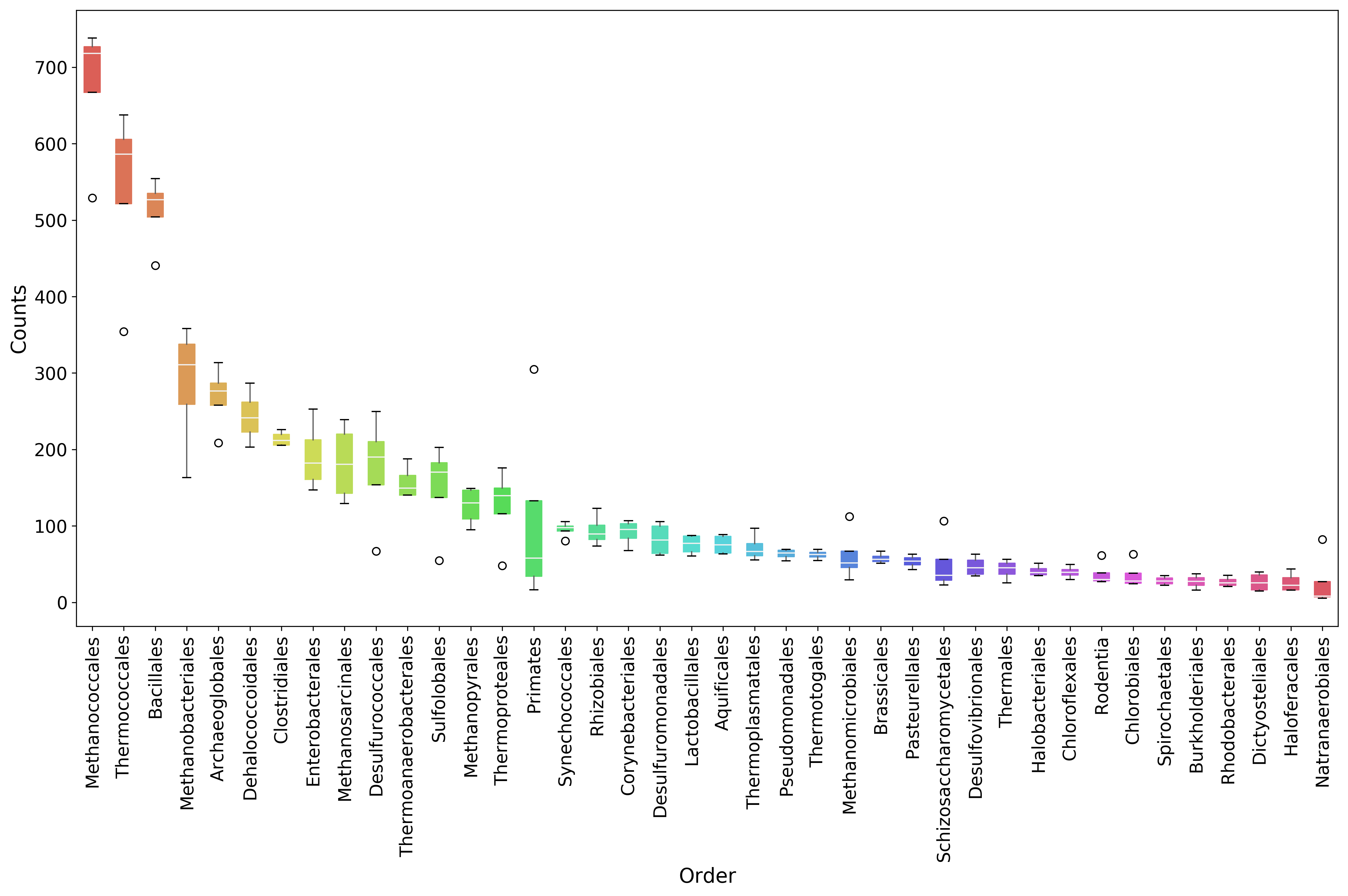
Plots for Top40 Taxa
Distribution of Each Taxon Over Depth
How to visualise the data depends on the question we want to ask and the experimental design. As a starting point, it may be interesting to visualise the variation of a taxonomic order abundance over the samples. This can be done using boxplots, among other methods.
MGKit offers a few functions to make complex plots, with a starting point in mgkit.plots.boxplot.boxplot_dataframe. However, as the data produced is in fact a pandas DataFrame, which is widely supported, a host of different specialised libraries tht offer similar functions can be used.
[18]:
# A matplotlib Figure instance and a single axis can be returned
# by this MGKit function. It is an helper function, the axis is
# needed to plot and the figure object to save the file to disk
fig, ax = mgkit.plots.get_single_figure(figsize=(15, 10))
# The return value of mgkit.plots.boxplot.boxplot_dataframe is
# passed to the **_** special variable, as it is not needed and
# it would be printed, otherwise
_ = mgkit.plots.boxplot.boxplot_dataframe(
    # The full dataframe can be passed
    taxa_counts,
    # this variable is used to tell the function
    # which rows and in which order they need to
    # be plot. In this case only the first 40 are
    # plot
    taxa_counts.index[:40],
    # A matplotlib axis instance
    ax,
    # a dictionary with options related to the labels
    # on both the X and Y axes. In this case it changes
    # the size of the labels
    fonts=dict(fontsize=14),
    # The default is to use the same colors for all
    # boxes. A dictionary can be passed to change this
    # in this case, the 'hls' palette from seaborn is
    # used.
    data_colours={
        x: color
        for x, color in zip(taxa_counts.index[:40], seaborn.color_palette('hls', 40))
    }
)
# Adds labels to the axes
ax.set_xlabel('Order', fontsize=16)
ax.set_ylabel('Counts', fontsize=16)
# Ensure the correct layout before writing to disk
fig.set_tight_layout(True)
# Saves a PDF file, or any other supported format by matplotlib
fig.savefig('{}taxa_counts-boxplot_top40_taxa.pdf'.format(data_dir))
2018-05-22 14:06:28,310 - DEBUG - matplotlib.font_manager->findfont: findfont: Matching :family=sans-serif:style=normal:variant=normal:weight=normal:stretch=normal:size=14.0 to DejaVu Sans (u'/home/frubino/mgkit/dev-env/local/lib/python2.7/site-packages/matplotlib/mpl-data/fonts/ttf/DejaVuSans.ttf') with score of 0.050000
2018-05-22 14:06:28,357 - DEBUG - matplotlib.font_manager->findfont: findfont: Matching :family=sans-serif:style=normal:variant=normal:weight=normal:stretch=normal:size=16.0 to DejaVu Sans (u'/home/frubino/mgkit/dev-env/local/lib/python2.7/site-packages/matplotlib/mpl-data/fonts/ttf/DejaVuSans.ttf') with score of 0.050000
2018-05-22 14:06:28,386 - DEBUG - matplotlib.backends.backend_pdf->fontName: Assigning font /F1 = u'/home/frubino/mgkit/dev-env/local/lib/python2.7/site-packages/matplotlib/mpl-data/fonts/ttf/DejaVuSans.ttf'
2018-05-22 14:06:28,537 - DEBUG - matplotlib.backends.backend_pdf->writeFonts: Embedding font /home/frubino/mgkit/dev-env/local/lib/python2.7/site-packages/matplotlib/mpl-data/fonts/ttf/DejaVuSans.ttf.
2018-05-22 14:06:28,538 - DEBUG - matplotlib.backends.backend_pdf->writeFonts: Writing TrueType font.
/home/frubino/mgkit/dev-env/local/lib/python2.7/site-packages/matplotlib/figure.py:2267: UserWarning: This figure includes Axes that are not compatible with tight_layout, so results might be incorrect.
  warnings.warn("This figure includes Axes that are not compatible "
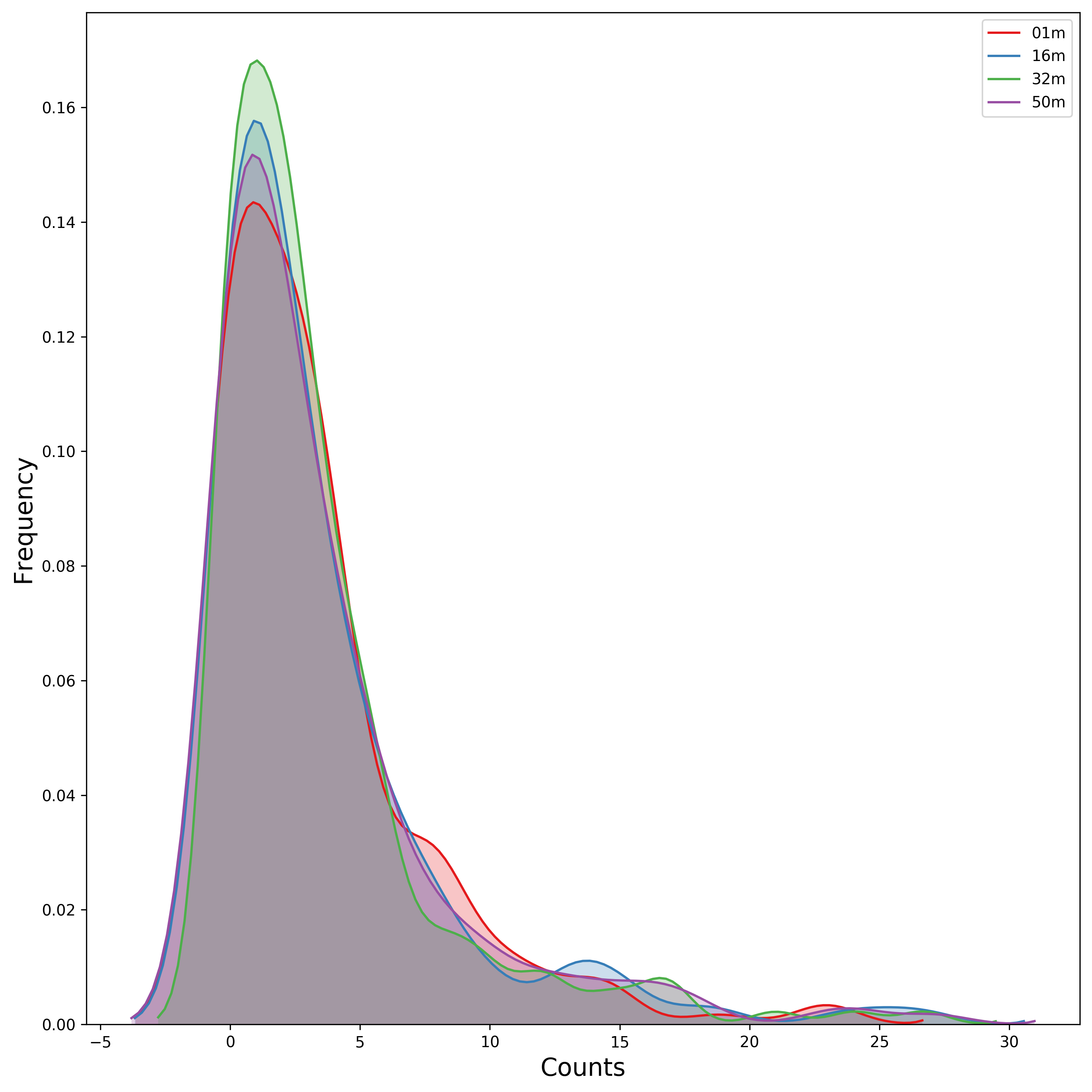
Distribution of Taxa at Each Depth
Seaborn offers a KDE plot, which is useful to display the distribution of taxa counts for each sampling depth.
[19]:
fig, ax = mgkit.plots.get_single_figure(figsize=(10, 10))
# iterate over the columns, which are the samples and assign a color to each one
for column, color in zip(taxa_counts.columns, seaborn.color_palette('Set1', len(taxa_counts.columns))):
    seaborn.kdeplot(
        # The data can transformed with the sqrt function of numpy
        numpy.sqrt(taxa_counts[column]),
        # Assign the color
        color=color,
        # Assign the label to the sample name to appear
        # in the legend
        label=column,
        # Add a shade under the KDE function
        shade=True
    )
# Adds a legend
ax.legend()
ax.set_xlabel('Counts', fontsize=16)
ax.set_ylabel('Frequency', fontsize=16)
fig.set_tight_layout(True)
fig.savefig('{}taxa_counts-distribution_top40_taxa.pdf'.format(data_dir))
2018-05-22 14:06:32,367 - DEBUG - matplotlib.font_manager->findfont: findfont: Matching :family=sans-serif:style=normal:variant=normal:weight=normal:stretch=normal:size=10.0 to DejaVu Sans (u'/home/frubino/mgkit/dev-env/local/lib/python2.7/site-packages/matplotlib/mpl-data/fonts/ttf/DejaVuSans.ttf') with score of 0.050000
2018-05-22 14:06:32,404 - DEBUG - matplotlib.backends.backend_pdf->fontName: Assigning font /F1 = u'/home/frubino/mgkit/dev-env/local/lib/python2.7/site-packages/matplotlib/mpl-data/fonts/ttf/DejaVuSans.ttf'
2018-05-22 14:06:32,461 - DEBUG - matplotlib.backends.backend_pdf->writeFonts: Embedding font /home/frubino/mgkit/dev-env/local/lib/python2.7/site-packages/matplotlib/mpl-data/fonts/ttf/DejaVuSans.ttf.
2018-05-22 14:06:32,463 - DEBUG - matplotlib.backends.backend_pdf->writeFonts: Writing TrueType font.
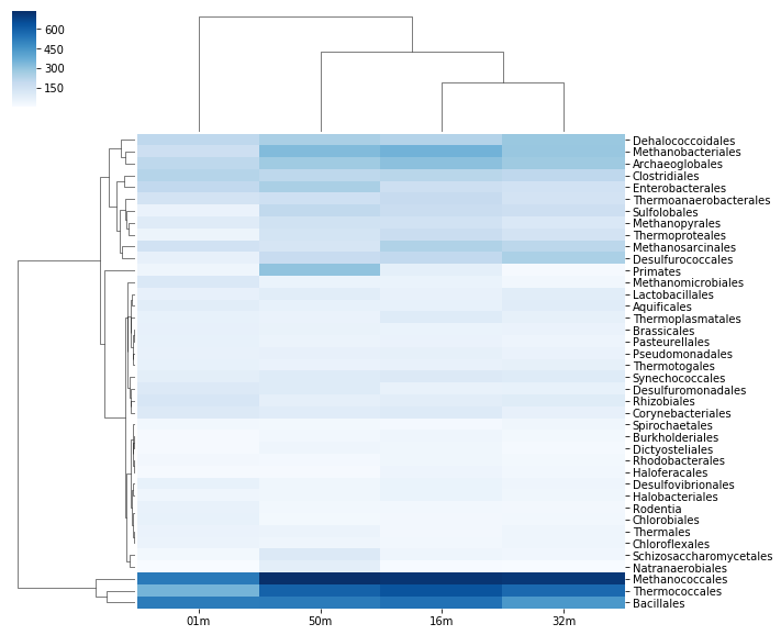
Heatmap of the Table
[20]:
# An heatmap can be created to provide information on the table
clfig = seaborn.clustermap(taxa_counts.iloc[:40], cbar=True, cmap='Blues')
clfig.fig.set_tight_layout(True)
for text in clfig.ax_heatmap.get_yticklabels():
    text.set_rotation('horizontal')
clfig.savefig('{}taxa_counts-heatmap-top40.pdf'.format(data_dir))
2018-05-22 14:06:34,833 - DEBUG - matplotlib.backends.backend_pdf->fontName: Assigning font /F1 = u'/home/frubino/mgkit/dev-env/local/lib/python2.7/site-packages/matplotlib/mpl-data/fonts/ttf/DejaVuSans.ttf'
2018-05-22 14:06:34,936 - DEBUG - matplotlib.backends.backend_pdf->writeFonts: Embedding font /home/frubino/mgkit/dev-env/local/lib/python2.7/site-packages/matplotlib/mpl-data/fonts/ttf/DejaVuSans.ttf.
2018-05-22 14:06:34,938 - DEBUG - matplotlib.backends.backend_pdf->writeFonts: Writing TrueType font.
2018-05-22 14:06:35,020 - DEBUG - matplotlib.backends.backend_pdf->fontName: Assigning font /F1 = u'/home/frubino/mgkit/dev-env/local/lib/python2.7/site-packages/matplotlib/mpl-data/fonts/ttf/DejaVuSans.ttf'
2018-05-22 14:06:35,129 - DEBUG - matplotlib.backends.backend_pdf->writeFonts: Embedding font /home/frubino/mgkit/dev-env/local/lib/python2.7/site-packages/matplotlib/mpl-data/fonts/ttf/DejaVuSans.ttf.
2018-05-22 14:06:35,131 - DEBUG - matplotlib.backends.backend_pdf->writeFonts: Writing TrueType font.
Functional Categories
Besides looking at specific taxa, it is possible to map each gene_id to functional categories. eggNOG provides this. v3 must be used, as the mappings in Uniprot points to that version.
Load Necessary Data
[21]:
eg = eggnog.NOGInfo()
[39]:
#Build mapping Uniprot IDs -> eggNOG functional categories
fc_map = {
    # An Annotation instance provide a method to access the list of IDs for the
    # specific mapping. For example eggnog mappings are store into the
    # map_EGGNOG attribute
    annotation.gene_id: eg.get_nogs_funccat(annotation.get_mapping('eggnog'))
    for annotation in annotations.itervalues()
}
[41]:
# Just a few to speed up the analysis, but other can be used
# Should have been downloaded by the full tutorial script
eg.load_members('{}COG.members.txt.gz'.format(data_dir))
eg.load_members('{}NOG.members.txt.gz'.format(data_dir))
eg.load_funccat('{}COG.funccat.txt.gz'.format(data_dir))
eg.load_funccat('{}NOG.funccat.txt.gz'.format(data_dir))
2018-05-22 14:09:38,473 - INFO - mgkit.mappings.eggnog->load_members: Reading Members from tutorial-data/COG.members.txt.gz
2018-05-22 14:09:56,921 - INFO - mgkit.mappings.eggnog->load_members: Reading Members from tutorial-data/NOG.members.txt.gz
2018-05-22 14:10:03,884 - INFO - mgkit.mappings.eggnog->load_funccat: Reading Functional Categories from tutorial-data/COG.funccat.txt.gz
2018-05-22 14:10:03,896 - INFO - mgkit.mappings.eggnog->load_funccat: Reading Functional Categories from tutorial-data/NOG.funccat.txt.gz
Build FC Table
As mentioned above, mgkit.counts.load_sample_counts_to_genes works in the same way as mgkit.counts.load_sample_counts_to_taxon, with the difference of giving gene_id as the only index.
In this case, however, as a mapping to functional categories is wanted, to the gene_map parameter a dictionary where for each gene_id an iterable of mappings is assigned. These are the values used in the index of the returned pandas.Series, which ends up as rows in the fc_counts DataFrame.
[45]:
fc_counts = pandas.DataFrame({
    file_name_to_sample(file_name): mgkit.counts.load_sample_counts_to_genes(
        lambda x: (annotations[x].gene_id, annotations[x].taxon_id),
        mgkit.counts.load_htseq_counts(file_name),
        taxonomy,
        gene_map=fc_map
    )
    for file_name in counts
})
2018-05-22 14:10:11,210 - INFO - mgkit.counts.func->load_htseq_counts: Loading HTSeq-count file tutorial-data/SRR001322-counts.txt
2018-05-22 14:10:11,293 - INFO - mgkit.counts.func->load_htseq_counts: Loading HTSeq-count file tutorial-data/SRR001323-counts.txt
2018-05-22 14:10:11,370 - INFO - mgkit.counts.func->load_htseq_counts: Loading HTSeq-count file tutorial-data/SRR001325-counts.txt
2018-05-22 14:10:11,445 - INFO - mgkit.counts.func->load_htseq_counts: Loading HTSeq-count file tutorial-data/SRR001326-counts.txt
Scale the Table and Rename Rows/Columns
[46]:
fc_counts = mgkit.counts.scale_deseq(fc_counts).rename(
    columns=sample_names,
    index=eggnog.EGGNOG_CAT
)
[47]:
fc_counts.describe()
[47]:
| 16m | 32m | 01m | 50m | |
|---|---|---|---|---|
| count | 23.000000 | 23.000000 | 23.000000 | 23.000000 |
| mean | 288.923364 | 289.089215 | 255.206073 | 287.413551 |
| std | 288.130525 | 286.446124 | 205.412833 | 283.111728 |
| min | 0.000000 | 0.000000 | 0.000000 | 3.471907 |
| 25% | 66.085234 | 78.138939 | 111.201303 | 69.004160 |
| 50% | 209.794392 | 232.510989 | 220.994995 | 223.070050 |
| 75% | 356.650467 | 388.026535 | 344.864801 | 376.701953 |
| max | 1103.518503 | 1147.308320 | 734.773169 | 1177.844584 |
[49]:
fc_counts
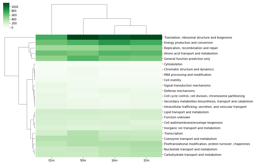
[49]:
| 16m | 32m | 01m | 50m | |
|---|---|---|---|---|
| RNA processing and modification | 4.195888 | 3.049324 | 25.337006 | 45.134796 |
| Chromatin structure and dynamics | 27.273271 | 21.345271 | 12.668503 | 68.570171 |
| Energy production and conversion | 832.883737 | 735.649521 | 609.495751 | 703.061248 |
| Cell cycle control, cell division, chromosome partitioning | 73.428037 | 97.578382 | 121.054583 | 52.078611 |
| Amino acid transport and metabolism | 676.586915 | 658.654079 | 609.495751 | 574.600674 |
| Nucleotide transport and metabolism | 336.719999 | 374.304575 | 271.669007 | 291.640221 |
| Carbohydrate transport and metabolism | 333.573084 | 354.483966 | 285.745121 | 275.148661 |
| Coenzyme transport and metabolism | 323.083364 | 304.170113 | 368.794196 | 374.098022 |
| Lipid transport and metabolism | 232.871775 | 238.609637 | 243.516778 | 243.901495 |
| Translation, ribosomal structure and biogenesis | 1103.518503 | 1147.308320 | 734.773169 | 1177.844584 |
| Transcription | 290.565233 | 276.726193 | 237.886332 | 365.418254 |
| Replication, recombination and repair | 528.681868 | 554.214717 | 439.174767 | 451.347962 |
| Cell wall/membrane/envelope biogenesis | 206.647476 | 174.573824 | 216.772161 | 199.634675 |
| Cell motility | 27.273271 | 19.058278 | 33.782674 | 33.851097 |
| Posttranslational modification, protein turnover, chaperones | 376.580934 | 401.748495 | 320.935407 | 379.305883 |
| Inorganic ion transport and metabolism | 186.717009 | 200.493082 | 190.027544 | 173.595370 |
| Secondary metabolites biosynthesis, transport and catabolism | 58.742430 | 86.143415 | 106.978469 | 96.345430 |
| General function prediction only | 577.983550 | 563.362690 | 494.071613 | 675.285989 |
| Function unknown | 209.794392 | 232.510989 | 220.994995 | 223.070050 |
| Signal transduction mechanisms | 35.665047 | 38.116555 | 115.424138 | 46.870750 |
| Intracellular trafficking, secretion, and vesicular transport | 87.064673 | 96.816051 | 121.054583 | 86.797685 |
| Defense mechanisms | 115.386916 | 70.134462 | 90.087132 | 69.438148 |
| Cytoskeleton | 0.000000 | 0.000000 | 0.000000 | 3.471907 |
[48]:
#Save table to disk
fc_counts.to_csv('{}fc_counts.csv'.format(data_dir))
Heatmap to Explore Functional Categories
[50]:
clfig = seaborn.clustermap(fc_counts, cbar=True, cmap='Greens')
clfig.fig.set_tight_layout(True)
for text in clfig.ax_heatmap.get_yticklabels():
    text.set_rotation('horizontal')
clfig.savefig('{}fc_counts-heatmap.pdf'.format(data_dir))
2018-05-22 14:10:17,521 - DEBUG - matplotlib.backends.backend_pdf->fontName: Assigning font /F1 = u'/home/frubino/mgkit/dev-env/local/lib/python2.7/site-packages/matplotlib/mpl-data/fonts/ttf/DejaVuSans.ttf'
2018-05-22 14:10:17,626 - DEBUG - matplotlib.backends.backend_pdf->writeFonts: Embedding font /home/frubino/mgkit/dev-env/local/lib/python2.7/site-packages/matplotlib/mpl-data/fonts/ttf/DejaVuSans.ttf.
2018-05-22 14:10:17,627 - DEBUG - matplotlib.backends.backend_pdf->writeFonts: Writing TrueType font.
2018-05-22 14:10:17,693 - DEBUG - matplotlib.backends.backend_pdf->fontName: Assigning font /F1 = u'/home/frubino/mgkit/dev-env/local/lib/python2.7/site-packages/matplotlib/mpl-data/fonts/ttf/DejaVuSans.ttf'
2018-05-22 14:10:17,798 - DEBUG - matplotlib.backends.backend_pdf->writeFonts: Embedding font /home/frubino/mgkit/dev-env/local/lib/python2.7/site-packages/matplotlib/mpl-data/fonts/ttf/DejaVuSans.ttf.
2018-05-22 14:10:17,799 - DEBUG - matplotlib.backends.backend_pdf->writeFonts: Writing TrueType font.
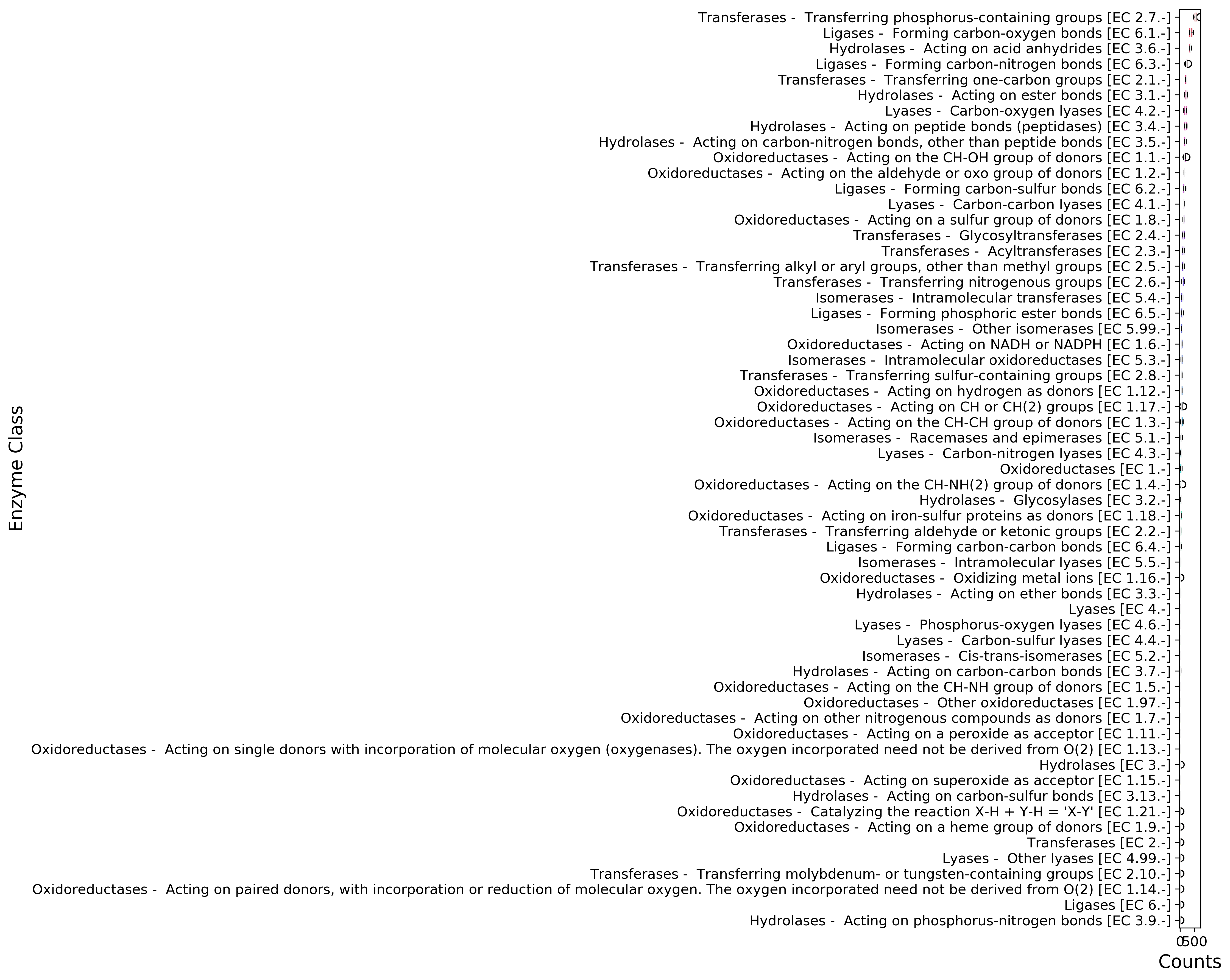
Enzyme Classification
Enzyme classification number were added the add-gff-info script, so they can be used in a similar way to functional categories. The specificity level requested is 2.
[51]:
ec_map = {
    # EC numbers are store into the EC attribute in a GFF file and
    # an Annotation instance provide a get_ec method that returns
    # a list. A level of specificity can be used to the mapping
    # less specific, as it ranges from 1 to 4 included. Right
    # now a list is returned, so it is a good idea to convert
    # the list into a set so if any duplicate appears (as effect
    # of the change in level) it won't inflate the number later.
    # In later versions (0.2) a set will be returned instead of
    # a list.
    # We also want to remove any hanging ".-" to use the labels
    # from expasy
    annotation.gene_id: set(x.replace('.-', '') for x in annotation.get_ec(level=2))
    for annotation in annotations.itervalues()
}
[52]:
# The only difference with the functional categories is the mapping
# used.
ec_counts = pandas.DataFrame({
    file_name_to_sample(file_name): mgkit.counts.load_sample_counts_to_genes(
        lambda x: (annotations[x].gene_id, annotations[x].taxon_id),
        mgkit.counts.load_htseq_counts(file_name),
        taxonomy,
        gene_map=ec_map
    )
    for file_name in counts
})
2018-05-22 14:10:20,682 - INFO - mgkit.counts.func->load_htseq_counts: Loading HTSeq-count file tutorial-data/SRR001322-counts.txt
2018-05-22 14:10:20,768 - INFO - mgkit.counts.func->load_htseq_counts: Loading HTSeq-count file tutorial-data/SRR001323-counts.txt
2018-05-22 14:10:20,844 - INFO - mgkit.counts.func->load_htseq_counts: Loading HTSeq-count file tutorial-data/SRR001325-counts.txt
2018-05-22 14:10:20,922 - INFO - mgkit.counts.func->load_htseq_counts: Loading HTSeq-count file tutorial-data/SRR001326-counts.txt
[53]:
# This file contains the names of each enzyme class and can be downloaded
# from ftp://ftp.expasy.org/databases/enzyme/enzclass.txt
# It should be downloaded at the end of the tutorial script
ec_names = mgkit.mappings.enzyme.parse_expasy_file('{}enzclass.txt'.format(data_dir))
[54]:
# Rename columns and row. Rows will include the full label the enzyme class
ec_counts = mgkit.counts.scale_deseq(ec_counts).rename(
    index=lambda x: "{} {} [EC {}.-]".format(
        # A name of the second level doesn't include the first level
        # definition, so if it is level 2, we add the level 1 label
        '' if len(x) == 1 else ec_names[x[0]] + " - ",
        # The EC label for the specific class (e.g. 3.2)
        ec_names[x],
        # The EC number
        x
    ),
    columns=sample_names
)
[55]:
plot_order = ec_counts.median(axis=1).sort_values(ascending=True, inplace=False).index
[56]:
ec_counts.describe()
[56]:
| 16m | 32m | 01m | 50m | |
|---|---|---|---|---|
| count | 59.000000 | 59.000000 | 59.000000 | 59.000000 |
| mean | 74.276636 | 78.371254 | 79.636608 | 80.406521 |
| std | 98.400500 | 108.265549 | 108.003831 | 115.948168 |
| min | 0.000000 | 0.000000 | 0.000000 | 0.000000 |
| 25% | 4.786284 | 6.764489 | 5.672632 | 3.995495 |
| 50% | 36.375758 | 42.090153 | 34.035791 | 37.291289 |
| 75% | 96.204307 | 105.225384 | 127.229027 | 121.640634 |
| max | 465.226796 | 537.401066 | 546.193404 | 674.794758 |
[57]:
ec_counts
[57]:
| 16m | 32m | 01m | 50m | |
|---|---|---|---|---|
| Oxidoreductases [EC 1.-] | 30.632217 | 18.038637 | 47.001806 | 64.815812 |
| Oxidoreductases - Acting on the CH-OH group of donors [EC 1.1.-] | 159.861883 | 134.538169 | 215.560008 | 161.595587 |
| Oxidoreductases - Acting on a peroxide as acceptor [EC 1.11.-] | 6.700797 | 14.280588 | 0.000000 | 3.551551 |
| Oxidoreductases - Acting on hydrogen as donors [EC 1.12.-] | 65.093461 | 81.173867 | 51.864062 | 46.170168 |
| Oxidoreductases - Acting on single donors with incorporation of molecular oxygen (oxygenases). The oxygen incorporated need not be derived from O(2) [EC 1.13.-] | 0.000000 | 7.516099 | 6.483008 | 3.551551 |
| Oxidoreductases - Acting on paired donors, with incorporation or reduction of molecular oxygen. The oxygen incorporated need not be derived from O(2) [EC 1.14.-] | 0.000000 | 0.000000 | 0.000000 | 1.775776 |
| Oxidoreductases - Acting on superoxide as acceptor [EC 1.15.-] | 4.786284 | 3.006440 | 0.000000 | 2.663664 |
| Oxidoreductases - Oxidizing metal ions [EC 1.16.-] | 14.358852 | 10.522538 | 3.241504 | 11.542542 |
| Oxidoreductases - Acting on CH or CH(2) groups [EC 1.17.-] | 54.563637 | 61.632010 | 102.107372 | 43.506504 |
| Oxidoreductases - Acting on iron-sulfur proteins as donors [EC 1.18.-] | 36.375758 | 15.783808 | 11.345264 | 37.291289 |
| Oxidoreductases - Acting on the aldehyde or oxo group of donors [EC 1.2.-] | 150.289315 | 145.812317 | 153.971434 | 139.398391 |
| Oxidoreductases - Catalyzing the reaction X-H + Y-H = 'X-Y' [EC 1.21.-] | 0.957257 | 6.012879 | 0.000000 | 0.000000 |
| Oxidoreductases - Acting on the CH-CH group of donors [EC 1.3.-] | 28.717703 | 42.090153 | 98.865868 | 63.927924 |
| Oxidoreductases - Acting on the CH-NH(2) group of donors [EC 1.4.-] | 36.375758 | 71.402939 | 30.794287 | 36.403401 |
| Oxidoreductases - Acting on the CH-NH group of donors [EC 1.5.-] | 0.957257 | 9.019319 | 16.207519 | 2.663664 |
| Oxidoreductases - Acting on NADH or NADPH [EC 1.6.-] | 71.794259 | 83.428697 | 53.484814 | 59.488485 |
| Oxidoreductases - Acting on other nitrogenous compounds as donors [EC 1.7.-] | 8.615311 | 0.000000 | 9.724512 | 1.775776 |
| Oxidoreductases - Acting on a sulfur group of donors [EC 1.8.-] | 125.400639 | 102.970554 | 111.831884 | 128.743737 |
| Oxidoreductases - Acting on a heme group of donors [EC 1.9.-] | 1.914514 | 0.000000 | 0.000000 | 0.000000 |
| Oxidoreductases - Other oxidoreductases [EC 1.97.-] | 1.914514 | 6.012879 | 4.862256 | 6.215215 |
| Transferases [EC 2.-] | 0.000000 | 0.000000 | 9.724512 | 0.000000 |
| Transferases - Transferring one-carbon groups [EC 2.1.-] | 192.408613 | 223.228135 | 222.043016 | 198.886876 |
| Transferases - Transferring molybdenum- or tungsten-containing groups [EC 2.10.-] | 0.000000 | 0.000000 | 3.241504 | 0.000000 |
| Transferases - Transferring aldehyde or ketonic groups [EC 2.2.-] | 27.760447 | 23.299906 | 21.069775 | 25.748747 |
| Transferases - Acyltransferases [EC 2.3.-] | 107.212760 | 126.270460 | 87.520605 | 146.501494 |
| Transferases - Glycosyltransferases [EC 2.4.-] | 82.324083 | 106.728603 | 129.660155 | 150.053045 |
| Transferases - Transferring alkyl or aryl groups, other than methyl groups [EC 2.5.-] | 79.452313 | 96.957675 | 147.488427 | 114.537531 |
| Transferases - Transferring nitrogenous groups [EC 2.6.-] | 85.195854 | 103.722164 | 144.246923 | 66.591588 |
| Transferases - Transferring phosphorus-containing groups [EC 2.7.-] | 465.226796 | 537.401066 | 546.193404 | 674.794758 |
| Transferases - Transferring sulfur-containing groups [EC 2.8.-] | 53.606380 | 60.880401 | 61.588574 | 71.031027 |
| Hydrolases [EC 3.-] | 2.871770 | 12.777368 | 3.241504 | 1.775776 |
| Hydrolases - Acting on ester bonds [EC 3.1.-] | 189.536843 | 239.763553 | 152.350682 | 227.299287 |
| Hydrolases - Acting on carbon-sulfur bonds [EC 3.13.-] | 0.000000 | 1.503220 | 6.483008 | 0.000000 |
| Hydrolases - Glycosylases [EC 3.2.-] | 39.247528 | 24.051516 | 47.001806 | 31.963962 |
| Hydrolases - Acting on ether bonds [EC 3.3.-] | 11.487081 | 9.019319 | 11.345264 | 9.766766 |
| Hydrolases - Acting on peptide bonds (peptidases) [EC 3.4.-] | 156.990112 | 190.157300 | 163.695946 | 233.514502 |
| Hydrolases - Acting on carbon-nitrogen bonds, other than peptide bonds [EC 3.5.-] | 203.895695 | 153.328416 | 149.109179 | 191.783773 |
| Hydrolases - Acting on acid anhydrides [EC 3.6.-] | 331.210847 | 338.224447 | 398.704977 | 350.715697 |
| Hydrolases - Acting on carbon-carbon bonds [EC 3.7.-] | 8.615311 | 1.503220 | 27.552783 | 4.439439 |
| Hydrolases - Acting on phosphorus-nitrogen bonds [EC 3.9.-] | 0.000000 | 0.000000 | 0.000000 | 4.439439 |
| Lyases [EC 4.-] | 2.871770 | 4.509659 | 12.966016 | 15.094093 |
| Lyases - Carbon-carbon lyases [EC 4.1.-] | 123.486125 | 131.531730 | 134.522411 | 107.434429 |
| Lyases - Carbon-oxygen lyases [EC 4.2.-] | 201.981181 | 171.367053 | 225.284520 | 133.183176 |
| Lyases - Carbon-nitrogen lyases [EC 4.3.-] | 50.734609 | 46.599813 | 27.552783 | 39.067065 |
| Lyases - Carbon-sulfur lyases [EC 4.4.-] | 13.401595 | 13.528978 | 0.000000 | 1.775776 |
| Lyases - Phosphorus-oxygen lyases [EC 4.6.-] | 15.316109 | 9.019319 | 4.862256 | 6.215215 |
| Lyases - Other lyases [EC 4.99.-] | 0.000000 | 0.000000 | 3.241504 | 0.000000 |
| Isomerases - Racemases and epimerases [EC 5.1.-] | 71.794259 | 51.861082 | 43.760302 | 31.076074 |
| Isomerases - Cis-trans-isomerases [EC 5.2.-] | 4.786284 | 9.770928 | 1.620752 | 14.206205 |
| Isomerases - Intramolecular oxidoreductases [EC 5.3.-] | 76.580543 | 50.357862 | 34.035791 | 78.134130 |
| Isomerases - Intramolecular transferases [EC 5.4.-] | 71.794259 | 92.448016 | 48.622558 | 85.237233 |
| Isomerases - Intramolecular lyases [EC 5.5.-] | 13.401595 | 5.261269 | 19.449023 | 15.981981 |
| Isomerases - Other isomerases [EC 5.99.-] | 84.238597 | 75.160988 | 59.967822 | 55.936934 |
| Ligases [EC 6.-] | 0.000000 | 0.000000 | 3.241504 | 0.000000 |
| Ligases - Forming carbon-oxygen bonds [EC 6.1.-] | 386.731740 | 450.214320 | 333.874900 | 338.285267 |
| Ligases - Forming carbon-sulfur bonds [EC 6.2.-] | 146.460288 | 129.276900 | 124.797899 | 190.895886 |
| Ligases - Forming carbon-nitrogen bonds [EC 6.3.-] | 218.254546 | 222.476525 | 270.665574 | 198.886876 |
| Ligases - Forming carbon-carbon bonds [EC 6.4.-] | 19.145136 | 19.541857 | 32.415039 | 6.215215 |
| Ligases - Forming phosphoric ester bonds [EC 6.5.-] | 44.991069 | 78.919038 | 68.071581 | 107.434429 |
[58]:
ec_counts.to_csv('{}ec_counts.csv'.format(data_dir))
[59]:
fig, ax = mgkit.plots.get_single_figure(figsize=(15, 12))
_ = mgkit.plots.boxplot.boxplot_dataframe(
    ec_counts,
    plot_order,
    ax,
    # a dictionary with options related to the labels
    # on both the X and Y axes. In this case it changes
    # the size of the labels and the rotation - the default
    # is 'vertical', as the box_vert=True by default
    fonts=dict(fontsize=12, rotation='horizontal'),
    data_colours={
        x: color
        for x, color in zip(plot_order, seaborn.color_palette('hls', len(plot_order)))
    },
    # Changes the direction of the boxplot. The rotation of
    # the labels must be set to 'horizontal' in the *fonts*
    # dictionary
    box_vert=False
)
# Adds labels to the axes
ax.set_xlabel('Counts', fontsize=16)
ax.set_ylabel('Enzyme Class', fontsize=16)
# Ensure the correct layout before writing to disk
fig.set_tight_layout(True)
# Saves a PDF file, or any other supported format by matplotlib
fig.savefig('{}ec_counts-boxplot.pdf'.format(data_dir))
2018-05-22 14:10:25,953 - DEBUG - matplotlib.font_manager->findfont: findfont: Matching :family=sans-serif:style=normal:variant=normal:weight=normal:stretch=normal:size=12.0 to DejaVu Sans (u'/home/frubino/mgkit/dev-env/local/lib/python2.7/site-packages/matplotlib/mpl-data/fonts/ttf/DejaVuSans.ttf') with score of 0.050000
2018-05-22 14:10:26,264 - DEBUG - matplotlib.backends.backend_pdf->fontName: Assigning font /F1 = u'/home/frubino/mgkit/dev-env/local/lib/python2.7/site-packages/matplotlib/mpl-data/fonts/ttf/DejaVuSans.ttf'
2018-05-22 14:10:26,958 - DEBUG - matplotlib.backends.backend_pdf->writeFonts: Embedding font /home/frubino/mgkit/dev-env/local/lib/python2.7/site-packages/matplotlib/mpl-data/fonts/ttf/DejaVuSans.ttf.
2018-05-22 14:10:26,960 - DEBUG - matplotlib.backends.backend_pdf->writeFonts: Writing TrueType font.
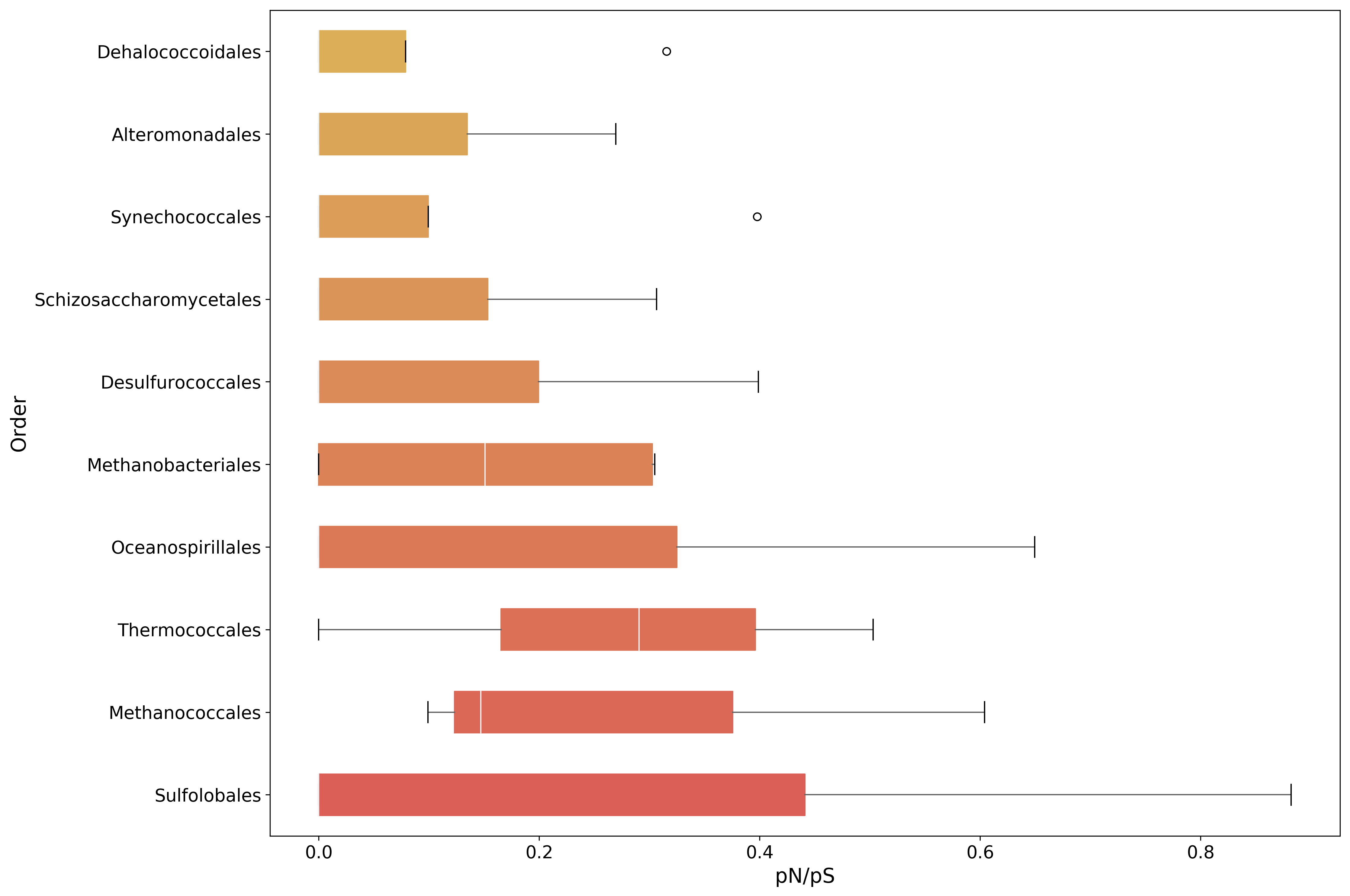
Explore Diversity
Diversity in metagenomic samples can be analysed using pN/pS values. The data required to do this was produced in the tutorial by the snp_parser script. Here are some examples of how to calculate diversity estimates from this data.
The complete toolset to map diversity estimates can be found in the mgkit.snps package, with the mgkit.snps.funcs.combine_sample_snps function building the final pandas DataFrame. As the use of the function requires the initialisation of different functions, a few easier to use ones are available in the mgkit.snps.conv_func module:
- get_rank_dataframe
- get_gene_map_dataframe
- get_full_dataframe
- get_gene_taxon_dataframe
The first is used to get diversity estimates for taxa, the second for genes/functions. The other two provides functionality to return estimates tied to both taxon and function.
Taxa
[60]:
# Sets the minimum coverage for an annotation to be
# included into the table (defaults to 4)
mgkit.consts.DEFAULT_SNP_FILTER['min_cov'] = 2
[61]:
# To get diversity estimates for taxa *mgkit.snps.conv_func.get_rank_dataframe* can be used
# It is also imported and accesible from the *mgkit.snps* package
pnps = mgkit.snps.get_rank_dataframe(snp_data, taxonomy, min_num=3, rank='order', index_type='taxon')
2018-05-22 14:10:34,437 - INFO - mgkit.snps.funcs->combine_sample_snps: Analysing SNP from sample SRR001322
2018-05-22 14:10:34,491 - INFO - mgkit.snps.funcs->combine_sample_snps: Analysing SNP from sample SRR001323
2018-05-22 14:10:34,552 - INFO - mgkit.snps.funcs->combine_sample_snps: Analysing SNP from sample SRR001325
2018-05-22 14:10:34,610 - INFO - mgkit.snps.funcs->combine_sample_snps: Analysing SNP from sample SRR001326
[62]:
pnps = pnps.rename(
    columns=sample_names,
    index=lambda x: taxonomy[x].s_name
)
[63]:
pnps.describe()
[63]:
| 16m | 32m | 01m | 50m | |
|---|---|---|---|---|
| count | 83.000000 | 83.000000 | 86.0 | 75.000000 |
| mean | 0.027889 | 0.035167 | 0.0 | 0.020063 |
| std | 0.086763 | 0.136137 | 0.0 | 0.100393 |
| min | 0.000000 | 0.000000 | 0.0 | 0.000000 |
| 25% | 0.000000 | 0.000000 | 0.0 | 0.000000 |
| 50% | 0.000000 | 0.000000 | 0.0 | 0.000000 |
| 75% | 0.000000 | 0.000000 | 0.0 | 0.000000 |
| max | 0.360621 | 0.882326 | 0.0 | 0.604127 |
[64]:
pnps
[64]:
| 16m | 32m | 01m | 50m | |
|---|---|---|---|---|
| Rubrobacterales | 0.000000 | 0.000000 | 0.0 | 0.000000 |
| Sphaerobacterales | 0.000000 | 0.000000 | 0.0 | NaN |
| Bifidobacteriales | 0.000000 | 0.000000 | 0.0 | 0.000000 |
| Micrococcales | 0.000000 | 0.000000 | 0.0 | 0.000000 |
| Neisseriales | 0.000000 | 0.000000 | 0.0 | 0.000000 |
| Micromonosporales | 0.000000 | NaN | 0.0 | 0.000000 |
| Pseudonocardiales | 0.000000 | 0.000000 | 0.0 | NaN |
| Streptomycetales | 0.000000 | 0.000000 | 0.0 | 0.000000 |
| Streptosporangiales | 0.000000 | 0.000000 | 0.0 | 0.000000 |
| Haloferacales | 0.000000 | 0.000000 | 0.0 | 0.000000 |
| Bacteroidales | 0.000000 | 0.000000 | 0.0 | 0.000000 |
| Mycoplasmatales | 0.000000 | 0.000000 | 0.0 | 0.000000 |
| Corynebacteriales | 0.000000 | 0.000000 | 0.0 | 0.000000 |
| Schizosaccharomycetales | 0.306546 | NaN | 0.0 | 0.000000 |
| Clostridiales | NaN | 0.000000 | 0.0 | 0.000000 |
| Rhodocyclales | 0.000000 | 0.000000 | 0.0 | NaN |
| Thiotrichales | NaN | 0.000000 | 0.0 | 0.000000 |
| Pseudomonadales | 0.000000 | 0.000000 | 0.0 | 0.000000 |
| Legionellales | 0.314474 | 0.000000 | 0.0 | 0.000000 |
| Chlamydiales | 0.000000 | 0.000000 | 0.0 | 0.000000 |
| Chroococcales | 0.000000 | 0.000000 | 0.0 | NaN |
| Methanobacteriales | 0.301844 | 0.304830 | 0.0 | 0.000000 |
| Planctomycetales | 0.000000 | 0.000000 | 0.0 | 0.000000 |
| Synechococcales | 0.000000 | 0.000000 | 0.0 | 0.397696 |
| Desulfovibrionales | 0.000000 | 0.000000 | 0.0 | 0.000000 |
| Cenarchaeales | 0.000000 | 0.000000 | NaN | 0.000000 |
| Oscillatoriales | 0.000000 | 0.000000 | 0.0 | 0.000000 |
| Methanococcales | 0.099162 | 0.147193 | NaN | 0.604127 |
| Spirochaetales | 0.000000 | 0.000000 | 0.0 | 0.000000 |
| Nostocales | 0.000000 | 0.000000 | 0.0 | NaN |
| ... | ... | ... | ... | ... |
| Herpetosiphonales | 0.000000 | 0.000000 | 0.0 | 0.000000 |
| Thermomicrobiales | 0.000000 | NaN | 0.0 | 0.000000 |
| Nitrospirales | 0.000000 | 0.000000 | 0.0 | 0.000000 |
| Campylobacterales | 0.000000 | 0.000000 | 0.0 | 0.000000 |
| Acidithiobacillales | 0.000000 | 0.000000 | 0.0 | 0.000000 |
| Parachlamydiales | 0.000000 | 0.000000 | 0.0 | NaN |
| Thermotogales | 0.000000 | 0.000000 | 0.0 | 0.000000 |
| Methanopyrales | 0.000000 | 0.000000 | 0.0 | 0.000000 |
| Solibacterales | 0.000000 | 0.000000 | 0.0 | NaN |
| Cellvibrionales | 0.000000 | 0.000000 | 0.0 | NaN |
| Natranaerobiales | 0.000000 | 0.000000 | 0.0 | 0.000000 |
| Gloeobacterales | 0.000000 | 0.000000 | 0.0 | 0.000000 |
| Methanocellales | 0.000000 | 0.000000 | 0.0 | 0.000000 |
| Aquificales | 0.000000 | 0.000000 | 0.0 | 0.000000 |
| Petrotogales | 0.000000 | 0.000000 | 0.0 | NaN |
| Eurotiales | 0.000000 | 0.000000 | 0.0 | 0.000000 |
| Chlorobiales | 0.000000 | 0.000000 | 0.0 | 0.000000 |
| Onygenales | NaN | 0.000000 | 0.0 | 0.000000 |
| Chromatiales | 0.000000 | 0.000000 | 0.0 | 0.000000 |
| Xanthomonadales | 0.000000 | 0.000000 | 0.0 | 0.000000 |
| Oceanospirillales | NaN | 0.649600 | 0.0 | 0.000000 |
| Flavobacteriales | 0.000000 | 0.000000 | 0.0 | 0.000000 |
| Alteromonadales | 0.269426 | NaN | 0.0 | 0.000000 |
| Vibrionales | 0.000000 | 0.000000 | 0.0 | 0.000000 |
| Aeromonadales | 0.000000 | 0.000000 | 0.0 | NaN |
| Pasteurellales | 0.299672 | 0.000000 | 0.0 | 0.000000 |
| Syntrophobacterales | 0.000000 | 0.000000 | 0.0 | 0.000000 |
| Rickettsiales | 0.000000 | 0.000000 | 0.0 | 0.000000 |
| Methanosarcinales | 0.059651 | NaN | 0.0 | 0.000000 |
| Cytophagales | 0.000000 | 0.000000 | 0.0 | NaN |
90 rows × 4 columns
[65]:
pnps.to_csv('{}pnps-taxa.csv'.format(data_dir))
[66]:
#sort the DataFrame to plot them by mean value
plot_order = pnps.mean(axis=1).sort_values(inplace=False, ascending=False).index[:10]

fig, ax = mgkit.plots.get_single_figure(figsize=(15, 10))
_ = mgkit.plots.boxplot.boxplot_dataframe(
    pnps,
    plot_order,
    ax,
    fonts=dict(fontsize=14, rotation='horizontal'),
    data_colours={
        x: color
        for x, color in zip(plot_order, seaborn.color_palette('hls', len(pnps.index)))
    },
    box_vert=False
)
ax.set_xlabel('pN/pS', fontsize=16)
ax.set_ylabel('Order', fontsize=16)
fig.set_tight_layout(True)
fig.savefig('{}pnps-taxa-boxplot.pdf'.format(data_dir))
/home/frubino/mgkit/dev-env/local/lib/python2.7/site-packages/numpy/core/fromnumeric.py:52: FutureWarning: reshape is deprecated and will raise in a subsequent release. Please use .values.reshape(...) instead
  return getattr(obj, method)(*args, **kwds)
2018-05-22 14:10:34,970 - DEBUG - matplotlib.backends.backend_pdf->fontName: Assigning font /F1 = u'/home/frubino/mgkit/dev-env/local/lib/python2.7/site-packages/matplotlib/mpl-data/fonts/ttf/DejaVuSans.ttf'
2018-05-22 14:10:35,015 - DEBUG - matplotlib.backends.backend_pdf->writeFonts: Embedding font /home/frubino/mgkit/dev-env/local/lib/python2.7/site-packages/matplotlib/mpl-data/fonts/ttf/DejaVuSans.ttf.
2018-05-22 14:10:35,016 - DEBUG - matplotlib.backends.backend_pdf->writeFonts: Writing TrueType font.
Functional Categories
[67]:
# To get diversity estimates of functions, *mgkit.snps.conv_func.get_gene_map_dataframe* can be used
# This is available in the *mgkit.snps* package as well
fc_pnps = mgkit.snps.get_gene_map_dataframe(snp_data, taxonomy, min_num=3, gene_map=fc_map, index_type='gene')
2018-05-22 14:10:38,138 - INFO - mgkit.snps.funcs->combine_sample_snps: Analysing SNP from sample SRR001322
2018-05-22 14:10:38,174 - INFO - mgkit.snps.funcs->combine_sample_snps: Analysing SNP from sample SRR001323
2018-05-22 14:10:38,215 - INFO - mgkit.snps.funcs->combine_sample_snps: Analysing SNP from sample SRR001325
2018-05-22 14:10:38,256 - INFO - mgkit.snps.funcs->combine_sample_snps: Analysing SNP from sample SRR001326
[68]:
fc_pnps = fc_pnps.rename(
    columns=sample_names,
    index=eggnog.EGGNOG_CAT
)
[69]:
fc_pnps.describe()
[69]:
| 16m | 32m | 01m | 50m | |
|---|---|---|---|---|
| count | 18.000000 | 15.000000 | 18.0 | 19.000000 |
| mean | 0.106591 | 0.195602 | 0.0 | 0.085110 |
| std | 0.149325 | 0.257863 | 0.0 | 0.173999 |
| min | 0.000000 | 0.000000 | 0.0 | 0.000000 |
| 25% | 0.000000 | 0.000000 | 0.0 | 0.000000 |
| 50% | 0.000000 | 0.076031 | 0.0 | 0.000000 |
| 75% | 0.275874 | 0.225485 | 0.0 | 0.127011 |
| max | 0.410372 | 0.761215 | 0.0 | 0.701625 |
[70]:
fc_pnps
[70]:
| 16m | 32m | 01m | 50m | |
|---|---|---|---|---|
| RNA processing and modification | NaN | 0.000000 | 0.0 | 0.000000 |
| Energy production and conversion | 0.300669 | 0.214854 | NaN | 0.201721 |
| Chromatin structure and dynamics | 0.000000 | 0.000000 | 0.0 | 0.000000 |
| Amino acid transport and metabolism | NaN | 0.060911 | 0.0 | 0.000000 |
| Cell cycle control, cell division, chromosome partitioning | 0.000000 | NaN | 0.0 | 0.000000 |
| Nucleotide transport and metabolism | 0.060956 | 0.236117 | 0.0 | 0.000000 |
| Lipid transport and metabolism | 0.000000 | NaN | 0.0 | 0.000000 |
| Coenzyme transport and metabolism | 0.410372 | 0.761215 | 0.0 | 0.302295 |
| Transcription | 0.306611 | 0.076031 | 0.0 | 0.000000 |
| Translation, ribosomal structure and biogenesis | 0.029312 | 0.048914 | NaN | 0.701625 |
| Cell wall/membrane/envelope biogenesis | 0.000000 | 0.601078 | 0.0 | NaN |
| Replication, recombination and repair | 0.306580 | 0.148139 | 0.0 | 0.000000 |
| Posttranslational modification, protein turnover, chaperones | 0.302645 | NaN | 0.0 | 0.102591 |
| Cell motility | 0.000000 | 0.000000 | 0.0 | 0.000000 |
| Secondary metabolites biosynthesis, transport and catabolism | 0.000000 | 0.000000 | 0.0 | 0.000000 |
| Inorganic ion transport and metabolism | 0.000000 | NaN | 0.0 | 0.157425 |
| Function unknown | 0.000000 | NaN | 0.0 | 0.000000 |
| General function prediction only | 0.201490 | 0.149640 | 0.0 | 0.151431 |
| Signal transduction mechanisms | 0.000000 | 0.000000 | 0.0 | 0.000000 |
| Defense mechanisms | 0.000000 | 0.637127 | 0.0 | 0.000000 |
[71]:
fc_pnps.to_csv('{}pnps-fc.csv'.format(data_dir))
[72]:
#sort the DataFrame to plot them by median value
plot_order = fc_pnps.mean(axis=1).sort_values(inplace=False, ascending=False).index

fig, ax = mgkit.plots.get_single_figure(figsize=(15, 10))
_ = mgkit.plots.boxplot.boxplot_dataframe(
    fc_pnps,
    plot_order,
    ax,
    fonts=dict(fontsize=14, rotation='horizontal'),
    data_colours={
        x: color
        for x, color in zip(plot_order, seaborn.color_palette('hls', len(fc_pnps.index)))
    },
    box_vert=False
)
ax.set_xlabel('pN/pS', fontsize=16)
ax.set_ylabel('Functional Category', fontsize=16)
fig.set_tight_layout(True)
fig.savefig('{}pnps-fc-boxplot.pdf'.format(data_dir))
2018-05-22 14:10:38,683 - DEBUG - matplotlib.backends.backend_pdf->fontName: Assigning font /F1 = u'/home/frubino/mgkit/dev-env/local/lib/python2.7/site-packages/matplotlib/mpl-data/fonts/ttf/DejaVuSans.ttf'
2018-05-22 14:10:38,777 - DEBUG - matplotlib.backends.backend_pdf->writeFonts: Embedding font /home/frubino/mgkit/dev-env/local/lib/python2.7/site-packages/matplotlib/mpl-data/fonts/ttf/DejaVuSans.ttf.
2018-05-22 14:10:38,778 - DEBUG - matplotlib.backends.backend_pdf->writeFonts: Writing TrueType font.
Enzyme Classification
[73]:
ec_map = {
    # Using only the first level
    annotation.gene_id: set(x.replace('.-', '') for x in annotation.get_ec(level=1))
    for annotation in annotations.itervalues()
}
[74]:
ec_pnps = mgkit.snps.get_gene_map_dataframe(snp_data, taxonomy, min_num=3, gene_map=ec_map, index_type='gene')
2018-05-22 14:10:42,201 - INFO - mgkit.snps.funcs->combine_sample_snps: Analysing SNP from sample SRR001322
2018-05-22 14:10:42,238 - INFO - mgkit.snps.funcs->combine_sample_snps: Analysing SNP from sample SRR001323
2018-05-22 14:10:42,277 - INFO - mgkit.snps.funcs->combine_sample_snps: Analysing SNP from sample SRR001325
2018-05-22 14:10:42,319 - INFO - mgkit.snps.funcs->combine_sample_snps: Analysing SNP from sample SRR001326
[75]:
# Rename columns and row. Rows will include the full label the enzyme class
ec_pnps = ec_pnps.rename(
    index=lambda x: "{} {} [EC {}.-]".format(
        # A name of the second level doesn't include the first level
        # definition, so if it is level 2, we add the level 1 label
        '' if len(x) == 1 else ec_names[x[0]] + " - ",
        # The EC label for the specific class (e.g. 3.2)
        ec_names[x],
        # The EC number
        x
    ),
    columns=sample_names
)
[76]:
ec_pnps.describe()
[76]:
| 16m | 32m | 01m | 50m | |
|---|---|---|---|---|
| count | 3.000000 | 3.000000 | 2.0 | 3.000000 |
| mean | 0.351120 | 0.187620 | 0.0 | 0.173303 |
| std | 0.248257 | 0.139590 | 0.0 | 0.185190 |
| min | 0.100278 | 0.100437 | 0.0 | 0.000000 |
| 25% | 0.228326 | 0.107119 | 0.0 | 0.075732 |
| 50% | 0.356374 | 0.113802 | 0.0 | 0.151464 |
| 75% | 0.476541 | 0.231211 | 0.0 | 0.259954 |
| max | 0.596708 | 0.348620 | 0.0 | 0.368444 |
[77]:
ec_pnps
[77]:
| 16m | 32m | 01m | 50m | |
|---|---|---|---|---|
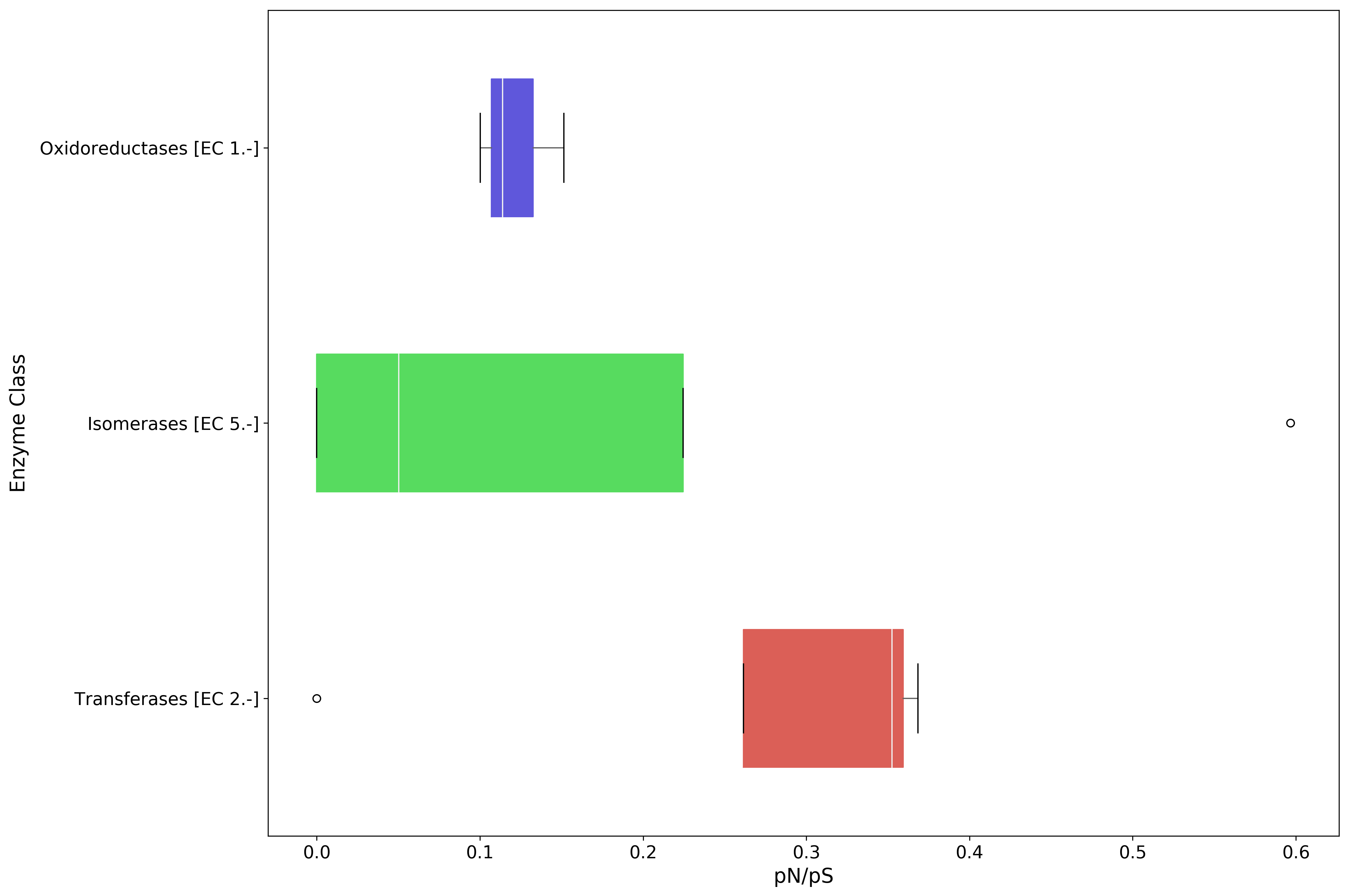
| Oxidoreductases [EC 1.-] | 0.100278 | 0.113802 | NaN | 0.151464 |
| Transferases [EC 2.-] | 0.356374 | 0.348620 | 0.0 | 0.368444 |
| Isomerases [EC 5.-] | 0.596708 | 0.100437 | 0.0 | 0.000000 |
[78]:
ec_pnps.to_csv('{}pnps-ec.csv'.format(data_dir))
[79]:
#sort the DataFrame to plot them by median value
plot_order = ec_pnps.mean(axis=1).sort_values(inplace=False, ascending=False).index

fig, ax = mgkit.plots.get_single_figure(figsize=(15, 10))
_ = mgkit.plots.boxplot.boxplot_dataframe(
    ec_pnps,
    plot_order,
    ax,
    fonts=dict(fontsize=14, rotation='horizontal'),
    data_colours={
        x: color
        for x, color in zip(plot_order, seaborn.color_palette('hls', len(plot_order)))
    },
    box_vert=False
)
ax.set_xlabel('pN/pS', fontsize=16)
ax.set_ylabel('Enzyme Class', fontsize=16)
fig.set_tight_layout(True)
fig.savefig('{}pnps-ec-boxplot.pdf'.format(data_dir))
2018-05-22 14:10:43,431 - DEBUG - matplotlib.backends.backend_pdf->fontName: Assigning font /F1 = u'/home/frubino/mgkit/dev-env/local/lib/python2.7/site-packages/matplotlib/mpl-data/fonts/ttf/DejaVuSans.ttf'
2018-05-22 14:10:43,455 - DEBUG - matplotlib.backends.backend_pdf->writeFonts: Embedding font /home/frubino/mgkit/dev-env/local/lib/python2.7/site-packages/matplotlib/mpl-data/fonts/ttf/DejaVuSans.ttf.
2018-05-22 14:10:43,456 - DEBUG - matplotlib.backends.backend_pdf->writeFonts: Writing TrueType font.